2026 · Master’s thesis, MSc in Big Data & Visual Analytics, UNIR · with Ikerlan
A wear bench that runs itself
A brass bushing wears out on a test bench at Ikerlan, about a tenth of a millimetre a day. I built the system around it that measures that wear, forecasts it and shows it live, with no one in the loop.
The problem
Every experiment needed a technician to move files, run scripts and draw plots by hand.
What I built
An event-driven pipeline, a backend and a dashboard, deployed as two Docker images.
What it showed
No purely data-driven model wins in every regime: the case for physics-informed ones.
Predicting a part’s death
Prognostics and health management (PHM) asks a simple question with an expensive answer: how long until this component fails? Answer it well and maintenance happens just before the failure, not after it, and not months too early on a schedule. Answering it needs sensor data processed as it arrives, a model of how the part degrades, and a way for engineers to see and trust what the model says.
Ikerlan’s AI & Data team studies this on a bench that reproduces a crank–slider mechanism, the same geometry that turns rotation into linear motion in engines, compressors and pumps. The part under study is the bushing in the joint between crank and rod. As it wears, the joint loosens.
Measuring wear without touching it
You cannot put a gauge inside a turning joint. But a looser joint lets the rod reach a little further, so the slider’s stroke grows with wear. A laser reading the slider’s position is therefore a soft sensor for the bushing: take the crest of each cycle, and the wear accumulated since the start is how far the crest has moved,
The crest moves by nanometres per cycle, far below the laser’s noise, so the raw estimate is jagged and the occasional acquisition glitch produces jumps no bushing could make. The wear module rejects those jumps and smooths what is left. Run the bench below to watch the estimate converge on the true wear.
Pick a component to see what it does. The amber tick under the slider marks how much further it now travels than at the start.
- Crest of each cycle
- Rejected as a glitch
- Wear estimate
- True wear
cycles (each stands for hours of a real experiment)
On the real bench, each experiment runs for about a week. The wear curves are far from the straight line a simple model would draw: a fast run-in while the surfaces bed in, long plateaus, sudden steps. After a week, one bushing has lost half a millimetre and another a full one.
Test 3. The sharpest run-in: 0.15 mm in the first few hours, then a slow, even climb to 0.7 mm.
Loading the curves…
A pipeline that waits for the bench
The acquisition software, LabVIEW, logs the motor, the laser and the load cell at 1 kHz into separate files, one set per five-minute block. Before my work, turning those files into a wear curve and a forecast was a manual job, and so was every change to a model or its parameters.
I wrote the pipeline as four Python modules driven by events rather than a schedule. It does nothing until a block is complete, processes it and then waits again, so the bench can stop, restart or change speed without anyone touching the software. Each module reads and writes plain files with a fixed format, which makes them swappable: a new wear estimator or model drops in without the rest noticing.
In the lab, every five minutes
Anywhere, as events arrive
Live signals skip the batch: LabVIEW → backend → dashboard over TCP, in under a second.
Python, lab PC
wear
Turns the laser signal into a wear curve.
- Takes the crest of the slider position in every cycle; wear is how far the crest has moved.
- Changes that are implausibly large for one step are flagged as anomalies and re-interpolated before smoothing.
The fiddliest step is the merge. The three sensors are logged by separate acquisition tasks whose clocks disagree by a fraction of a cycle, and a fraction of a cycle is the difference between the spring pulling and pushing. Since all three see the same motion, their peaks must coincide. The pipeline finds the peaks in each stream, matches them and shifts the streams until they line up.
- Laser position
- Load-cell force
- ×Detected peak
Forecasts that say how sure they are
Four architectures forecast the wear curve from the sensors: two recurrent networks (LSTM and GRU), a temporal convolutional network (TCN) and PatchTST, a transformer that reads the series in patches. The pipeline runs whichever one is selected, and I evaluated all four on the bench.
A point forecast is not enough to schedule maintenance on: you need to know how far to trust it. The predict module uses Monte Carlo dropout. Dropout, normally switched off after training, stays on, so each forward pass samples a slightly different network. Over passes,
the mean is the forecast and the spread says how much the sampled networks disagree. To score forecasts that come with a spread, RMSE is not enough, because it only looks at the mean. The continuous ranked probability score (CRPS) compares the whole predicted distribution with the value that actually happened,
and so rewards a forecast that is both close and honestly uncertain. For a forecast with no spread at all, it reduces to the absolute error.
Rows: hours of history the model sees. Columns: how far ahead it forecasts. Stronger colour: larger error (mm).
Modes won, out of 16
- PatchTST2
- LSTM1
- GRU6
- TCN7
Show as table
| Window | Horizon | PatchTST | LSTM | GRU | TCN |
|---|---|---|---|---|---|
| 24 h | 12 h | 0.05259 | 0.05020 | 0.02797 | 0.04653 |
| 24 h | 24 h | 0.09784 | 0.08428 | 0.06043 | 0.05425 |
| 24 h | 48 h | 0.11868 | 0.10218 | 0.09670 | 0.07978 |
| 24 h | 72 h | 0.16804 | 0.08844 | 0.08969 | 0.09942 |
| 48 h | 12 h | 0.07422 | 0.06587 | 0.02895 | 0.02570 |
| 48 h | 24 h | 0.10535 | 0.07661 | 0.05303 | 0.04025 |
| 48 h | 48 h | 0.06609 | 0.06028 | 0.04916 | 0.05445 |
| 48 h | 72 h | 0.13245 | 0.06536 | 0.04124 | 0.08282 |
| 72 h | 12 h | 0.02875 | 0.04888 | 0.02802 | 0.02444 |
| 72 h | 24 h | 0.02807 | 0.07090 | 0.04091 | 0.03405 |
| 72 h | 48 h | 0.08831 | 0.04335 | 0.04199 | 0.04822 |
| 72 h | 72 h | 0.04577 | 0.04537 | 0.04300 | 0.04685 |
| 96 h | 12 h | 0.04448 | 0.05058 | 0.04044 | 0.02883 |
| 96 h | 24 h | 0.02963 | 0.04281 | 0.02761 | 0.02836 |
| 96 h | 48 h | 0.02469 | 0.05008 | 0.06171 | 0.04497 |
| 96 h | 72 h | 0.09629 | 0.16323 | 0.11942 | 0.08122 |
No architecture wins everywhere. TCN is best in 7 of the 16 regimes on both metrics, GRU in 6 by RMSE, and PatchTST takes 4 by CRPS, mostly with long histories. The best error in a regime ranges from 0.024 to 0.088 mm, which against a millimetre of total wear means relative errors up to about 8 %. Errors grow with short histories and long horizons, exactly where a purely data-driven model has least to go on.
That last point is the real finding. Wear is governed by physics that is partly known: Archard’s law says the worn volume grows with the load and the sliding distance,
with a wear coefficient and the hardness of the softer material. Models that build this in and learn only what it leaves out (hybrid, physics-informed models) are the obvious next step. The environment exists to make testing them cheap.
Putting it in front of engineers
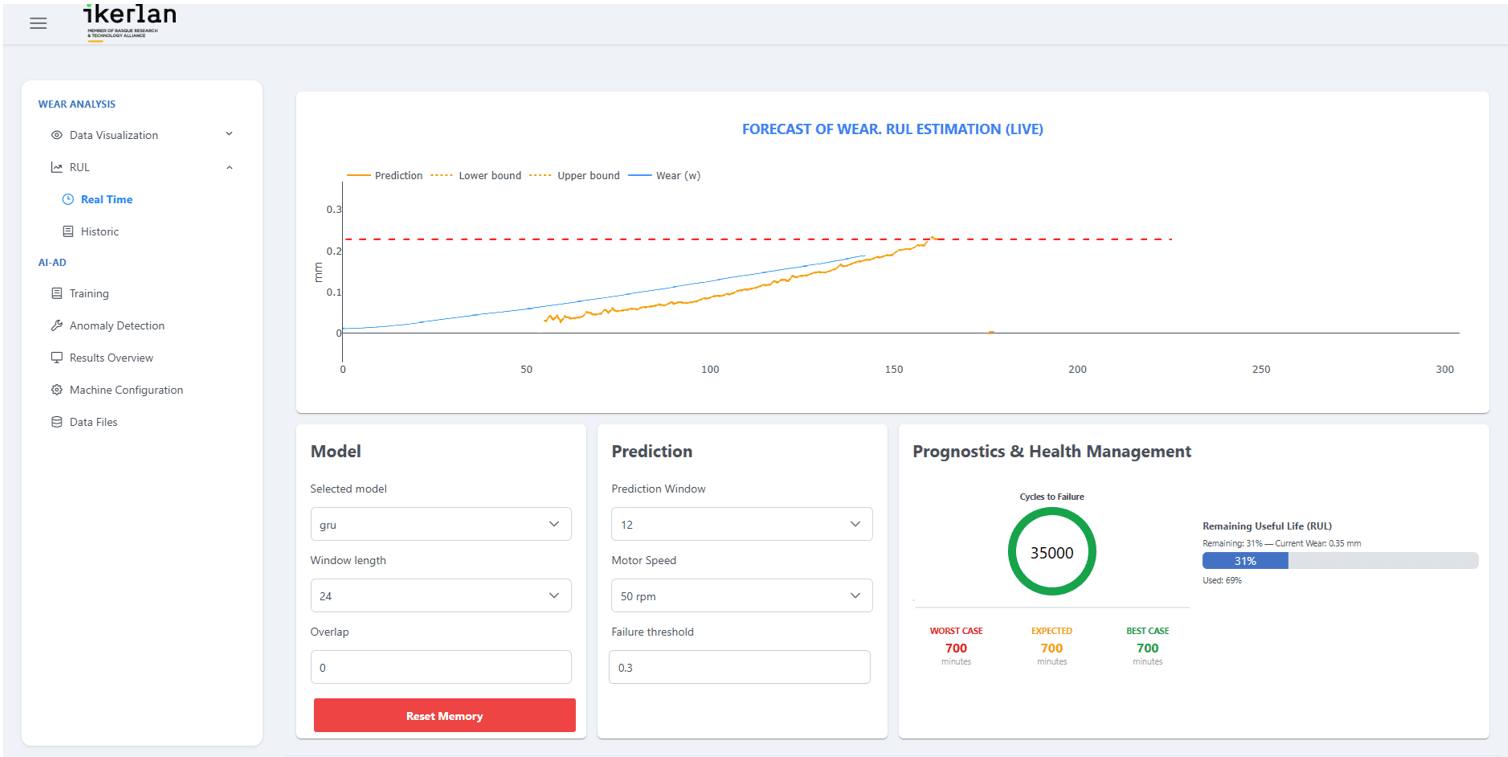
The dashboard is a React app talking to a Flask and Socket.IO backend. It shows the laser, motor and load cell live; the wear curve with the forecast and its band, against a failure threshold; a remaining-life estimate; and a history view to load past experiments and compare models with their metrics side by side. Control panels change the model, the window, the horizon and the bench speed, and the backend writes those changes back to the pipeline’s configuration.
Does it hold up?
I validated the whole environment with the research team on the real bench: signals in the dashboard identical to LabVIEW’s own, computed wear identical to what the pipeline wrote, and the system left running through pauses, restarts, gaps in the data and weeks of continuous operation.
< 2 min
to process each five-minute block
< 1 s
latency of the live signals
< 1 %
failed blocks in a week of running
1
exception in three weeks non-stop
Usability mattered as much: any setting takes one interaction to change, and loading a past experiment and adding it to a comparison takes four at most. Before, the same tasks needed someone who knew the code.
Limits and what comes next
The environment was designed and validated on one bench with one set of sensors, so carrying it to another machine would need its own validation. The hand-off from LabVIEW goes through files, which is robust and simple but adds latency that a faster process might not tolerate. And the models, as the matrix shows, are not yet accurate enough for an industrial decision.
What I take from it is the other half of doing science with data. A model is only as useful as the system that feeds it clean data on time and puts its answer, with its uncertainty, in front of the person who has to decide. It is the same discipline I now bring to brain-imaging data.
Tools. Python (pandas, NumPy, SciPy, PyTorch), Flask, Socket.IO, React, Docker, LabVIEW.
Data. All bench data belongs to Ikerlan and is not published here. The model metrics and wear curves are those reported in the thesis, the curves digitised from its figure; the bench and peak-alignment figures are simulations.
Credits. Master’s thesis for the MSc in Big Data & Visual Analytics at the Universidad Internacional de La Rioja (UNIR), carried out with the AI & Data department of Ikerlan.